深度强化学习算法

DQN

在之前我列举了几乎所有强化学习的公式,本期我们就针对如何应用这些公式进行讲解,传送门:强化学习基础

基础

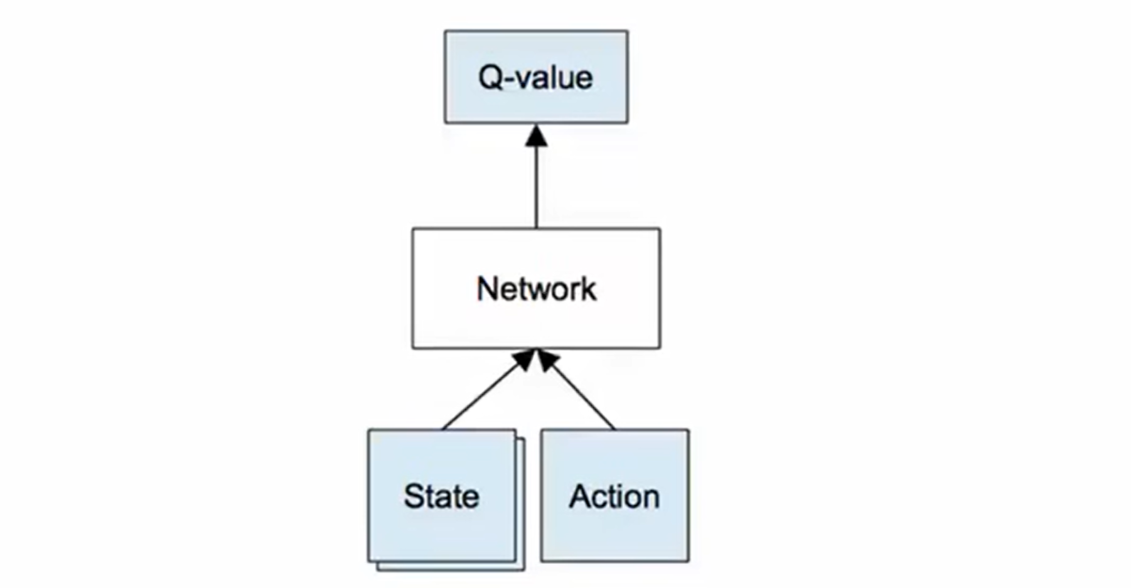
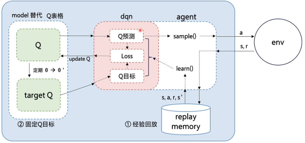
我们知道Q-Learning方法需要维护一张Q表格,本质上是把每个状态-动作对的价值都存下来。如果我们把这个Q表格用函数表达出来,就有了DQN的第一步思想。我们都知道,前馈神经网络的本质就是一个大型的函数,用它我们可以表达出复杂的价值函数,所以DQN就是将Q表格换成了可以计算价值的神经网络。

首先获取Q价值更新,其中Q函数是神经网络。

根据Q学习的公式我们可以使用最优贝尔曼方程定义出DQN的价值损失函数,我们可以用一般的反向传播算法进行计算。

在公式内:$Q_(s_t,a_t)$和$max_AQ_(s_{t+1},A)$是可计算的。我们就理解了DQN的神经网络是负责计算价值的。最终的输出为:

当然损失函数也可以用Y表示,也就是:

1

过程

  • 首先需要收集状态(s),并为每个行为(a)定义奖励(r),制定一个用于奖励回放的经验池。
  • 从经验池内抽出一组($s_t,a_t,r_t,s_{t+1}$)计算$Q(s_t,a_t)、max_AQ(s_{t+1},A)$
  • 使用损失函数计算损失值后进行反向传播

2

代码

我们用飞行小鸟做学习实例,注意python和tensorflow版本:

1
2
3
4
5
6
7
8
9
10
11
12
13
14
15
16
17
18
19
20
21
22
23
24
25
26
27
28
29
30
31
32
33
34
35
36
37
38
39
40
41
42
43
44
45
46
47
48
49
50
51
52
53
54
55
56
57
58
59
60
61
62
63
64
65
66
67
68
69
70
71
72
73
74
75
76
77
78
79
80
81
82
83
84
85
86
87
88
89
90
91
92
93
94
95
96
97
98
99
100
101
102
103
104
105
106
107
108
109
110
111
112
113
114
115
116
117
118
119
120
121
122
123
124
125
126
127
128
129
130
131
132
133
134
135
136
137
138
139
140
141
142
143
144
145
146
147
148
149
150
151
152
153
154
155
156
157
158
159
160
161
162
163
164
165
166
167
168
169
170
171
172
173
174
175
176
177
178
179
180
181
182
183
184
185
186
187
188
189
190
191
192
193
194
195
196
197
198
199
200
201
202
203
204
205
206
207
208
209
210
211
212
213
214
215
216
217
218
219
220
221
222
223
224
225
226
227
228
229
230
231
232
233
234
235
from __future__ import print_function

import tensorflow as tf
import cv2
import sys
sys.path.append("game/")
try:
from . import wrapped_flappy_bird as game
except Exception:
import wrapped_flappy_bird as game
import random
import numpy as np
from collections import deque

GAME = 'bird' # 日志目录名
ACTIONS = 2 # 往上1 往下0
GAMMA = 0.99 # 折扣因子
OBSERVE = 1000. # 先观察这些步, 只存经验不训练
EXPLORE = 3000000. # 探索衰减步数(epsilon 线性衰减)
FINAL_EPSILON = 0.0001 # 探索率下限
INITIAL_EPSILON = 0.0001 # 初始探索率
REPLAY_MEMORY = 50000 # 经验回放池容量
BATCH = 32 # 每次训练抽取的样本数
FRAME_PER_ACTION = 1

def weight_variable(shape):
initial = tf.truncated_normal(shape, stddev = 0.01)
return tf.Variable(initial)

def bias_variable(shape):
initial = tf.constant(0.01, shape = shape)
return tf.Variable(initial)
# padding--‘SAME’=> 图像尺寸/步长
# |-‘VALID’=> (图像尺寸-卷积核尺寸+1)/步
def conv2d(x, W, stride):
return tf.nn.conv2d(x, W, strides = [1, stride, stride, 1], padding = "SAME")

def max_pool_2x2(x):
return tf.nn.max_pool(x, ksize = [1, 2, 2, 1], strides = [1, 2, 2, 1], padding = "SAME")

def createNetwork():
# 权重
W_conv1 = weight_variable([8, 8, 4, 32])
b_conv1 = bias_variable([32])

W_conv2 = weight_variable([4, 4, 32, 64])
b_conv2 = bias_variable([64])

W_conv3 = weight_variable([3, 3, 64, 64])
b_conv3 = bias_variable([64])

W_fc1 = weight_variable([576, 512])
b_fc1 = bias_variable([512])

W_fc2 = weight_variable([512, ACTIONS])
b_fc2 = bias_variable([ACTIONS])

# 输入层
s = tf.placeholder("float", [None, 80, 80, 4])

# hidden layers
h_conv1 = tf.nn.relu(conv2d(s, W_conv1, 4) + b_conv1)
h_pool1 = max_pool_2x2(h_conv1)

h_conv2 = tf.nn.relu(conv2d(h_pool1, W_conv2, 2) + b_conv2)
h_pool2 = max_pool_2x2(h_conv2)

h_conv3 = tf.nn.relu(conv2d(h_conv2, W_conv3, 1) + b_conv3)
h_pool3 = max_pool_2x2(h_conv3)

h_pool3_flat = tf.reshape(h_pool3, [-1, 576])

h_fc1 = tf.nn.relu(tf.matmul(h_pool3_flat, W_fc1) + b_fc1)

# readout layer
readout = tf.matmul(h_fc1, W_fc2) + b_fc2

return s, readout, h_fc1

def trainNetwork(s, readout, h_fc1, sess):
# define the cost function
a = tf.placeholder("float", [None, ACTIONS])
y = tf.placeholder("float", [None])
# reduction_indices = axis 0 : 列 1: 行
# 因 y 是数值,而readout: 网络模型预测某个行为的回报 大小[1, 2]
# 所以用 tf.multiply(readout, a) 取出实际执行的那个行为的回报(one-hot 相乘),再求和。
readout_action = tf.reduce_mean(tf.multiply(readout, a), axis=1)
cost = tf.reduce_mean(tf.square(y - readout_action))
train_step = tf.train.AdamOptimizer(1e-6).minimize(cost)

# open up a game state to communicate with emulator
game_state = game.GameState()
# 创建队列保存参数
# store the previous observations in replay memory
D = deque()

# printing
a_file = open("logs_" + GAME + "/readout.txt", 'w')
h_file = open("logs_" + GAME + "/hidden.txt", 'w')

# get the first state by doing nothing and preprocess the image to 80x80x4
do_nothing = np.zeros(ACTIONS)
do_nothing[0] = 1
x_t, r_0, terminal = game_state.frame_step(do_nothing)
#cv2.imwrite('x_t.jpg',x_t)
x_t = cv2.cvtColor(cv2.resize(x_t, (80, 80)), cv2.COLOR_BGR2GRAY)
ret, x_t = cv2.threshold(x_t,1,255,cv2.THRESH_BINARY)
s_t = np.stack((x_t, x_t, x_t, x_t), axis=2)

# saving and loading networks
tf.summary.FileWriter("tensorboard/", sess.graph)
saver = tf.train.Saver()
sess.run(tf.initialize_all_variables())
checkpoint = tf.train.get_checkpoint_state("saved_networks")
# start training
epsilon = INITIAL_EPSILON
t = 0
while "flappy bird" != "angry bird":
# 预测结果(当前状态不同行为action的回报,其实也就 往上,往下 两种行为)
readout_t = readout.eval(feed_dict={s : [s_t]})[0]
a_t = np.zeros([ACTIONS])
action_index = 0
if t % FRAME_PER_ACTION == 0:
# 加入一些探索,比如探索一些相同回报下其他行为,可以提高模型的泛化能力。
# 且epsilon是随着模型稳定趋势衰减的,也就是模型越稳定,探索次数越少。
if random.random() <= epsilon:
# 在ACTIONS范围内随机选取一个作为当前状态的即时行为
print("----------Random Action----------")
action_index = random.randrange(ACTIONS)
a_t[action_index] = 1
else:
# 输出 奖励最大就是下一步的方向
action_index = np.argmax(readout_t)
a_t[action_index] = 1
else:
a_t[0] = 1 # do nothing

# 减少探索体的数量,可以保证模型稳定,减少探索次数。
if epsilon > FINAL_EPSILON and t > OBSERVE:
epsilon -= (INITIAL_EPSILON - FINAL_EPSILON) / EXPLORE

# 运行后进行观察,把
x_t1_colored, r_t, terminal = game_state.frame_step(a_t)
# 先将尺寸设置成 80 * 80,然后转换为灰度图
x_t1 = cv2.cvtColor(cv2.resize(x_t1_colored, (80, 80)), cv2.COLOR_BGR2GRAY)
# x_t1 新得到图像,二值化 阈值:1
ret, x_t1 = cv2.threshold(x_t1, 1, 255, cv2.THRESH_BINARY)
x_t1 = np.reshape(x_t1, (80, 80, 1))
#s_t1 = np.append(x_t1, s_t[:,:,1:], axis = 2)
# 取之前状态的前3帧图片 + 当前得到的1帧图片
# 每次输入都是4幅图像
s_t1 = np.append(x_t1, s_t[:, :, :3], axis=2)

# store the transition in D
# s_t: 当前状态(80 * 80 * 4)
# a_t: 即将行为 (1 * 2)
# r_t: 即时奖励
# s_t1: 下一状态
# terminal: 当前行动的结果(是否碰到障碍物 True => 是 False =>否)
# 保存参数,队列方式,超出上限,抛出最左端的元素。
D.append((s_t, a_t, r_t, s_t1, terminal))
if len(D) > REPLAY_MEMORY:
D.popleft()

# only train if done observing
if t > OBSERVE:
# 获取batch = 32个保存的参数集
minibatch = random.sample(D, BATCH)
# get the batch variables
# 获取j时刻batch(32)个状态state
s_j_batch = [d[0] for d in minibatch]
# 获取batch(32)个行动action
a_batch = [d[1] for d in minibatch]
# 获取保存的batch(32)个奖励reward
r_batch = [d[2] for d in minibatch]
# 获取保存的j + 1时刻的batch(32)个状态state
s_j1_batch = [d[3] for d in minibatch]
# readout_j1_batch =>(32, 2)
y_batch = []
readout_j1_batch = sess.run(readout, feed_dict = {s : s_j1_batch})
for i in range(0, len(minibatch)):
terminal = minibatch[i][4]
# if terminal, only equals reward
if terminal: # 碰到障碍物,终止
y_batch.append(r_batch[i])
else: # 即时奖励 + 下一阶段回报
y_batch.append(r_batch[i] + GAMMA * np.max(readout_j1_batch[i]))
# 根据cost -> 梯度 -> 反向传播 -> 更新参数
# perform gradient step
# 必须要3个参数,y, a, s 只是占位符,没有初始化
# 在 train_step过程中,需要这3个参数作为变量传入
train_step.run(feed_dict = {
y : y_batch,
a : a_batch,
s : s_j_batch}
)

# 更新值
s_t = s_t1 # state 更新
t += 1

# 保存10000的迭代
if t % 10000 == 0:
saver.save(sess, 'saved_networks/' + GAME + '-dqn', global_step = t)

state = ""
if t <= OBSERVE:
state = "observe"
elif t > OBSERVE and t <= OBSERVE + EXPLORE:
state = "explore"
else:
state = "train"

print("terminal", terminal, \
"TIMESTEP", t, "/ STATE", state, \
"/ EPSILON", epsilon, "/ ACTION", action_index, "/ REWARD", r_t, \
"/ Q_MAX %e" % np.max(readout_t))
# 写入文件
'''
if t % 10000 <= 100:
a_file.write(",".join([str(x) for x in readout_t]) + '\n')
h_file.write(",".join([str(x) for x in h_fc1.eval(feed_dict={s:[s_t]})[0]]) + '\n')
cv2.imwrite("logs_tetris/frame" + str(t) + ".png", x_t1)
'''

def playGame():
sess = tf.InteractiveSession()
s, readout, h_fc1 = createNetwork()
trainNetwork(s, readout, h_fc1, sess)

def main():
playGame()

if __name__ == "__main__":
main()

用大白话总结一下:ANN输出的Q是用于决策的,使用贝尔曼方程递推出来的Q是期望的Q,所以可以利用MSE进行训练神经网络,同时关注贝尔曼方程的递推方式。

DDQN

这里和DQN是一样的,唯一的区别就是计算目标Q时先选动作、再算价值,把选择和评估分开:

PPO

PPO是一种策略梯度算法,策略梯度不通过拟合价值误差来反向传播,而是根据回报直接调整动作被选中的概率:回报高的动作提高概率,低则降低。

提示,看不懂公式或者函数的话可以看这期文章:强化学习基础

基础

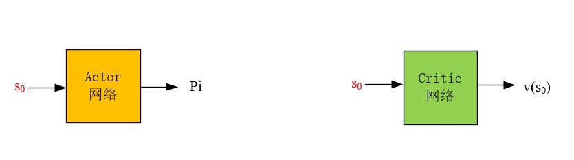
我们首先定义一下on-policy与off-policy也就是同轨策略和离轨策略:采样用的策略和正在改进的目标策略不是同一个,就是离轨策略;PPO 则是同轨策略。PPO方法定义了两个网络,分别负责将s计算为策略和价值:

3

Actor可以得到动作发生的概率,将动作放入环境里,就会得到对应的价值和下一个状态。Critic负责估计状态价值,价值估计用的是一条lambda回报,即:

如何更新Actor网络?我们看看它的定义:

因为是策略梯度,我们使用重要性采样:

则损失函数为:

其中的clip函数负责约束$\rho(\theta)$在区间($1-\epsilon,1+\epsilon$)内。通过此法可以更新Actor网络。Critic的更新就是拿算出来的回报作为目标去拟合价值函数。

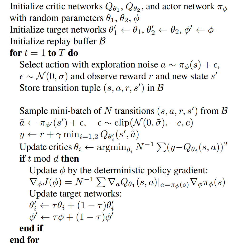
4

  • 实际行为a是Actor的输出加上一个高斯噪声
  • Critic网络最终的输出为:$y=r+\gamma minQ_t(s,a)$

  • 网络的损失为:$\nabla J(\theta)=\frac{1}{N}\sum_{i=1}^N(\sum_{t=1}^T \nabla \log\pi_\theta(a|s)(\sum_{t=1}^Tr(s,a)))$

  • 梯度更新

代码

1
2
3
4
5
6
7
8
9
10
11
12
13
14
15
16
17
18
19
20
21
22
23
24
25
26
27
28
29
30
31
32
33
34
35
36
37
38
39
40
41
42
43
44
45
46
47
48
49
50
51
52
53
54
55
56
57
58
59
60
61
62
63
64
65
66
67
68
69
70
71
72
73
74
75
76
77
78
79
80
81
82
83
84
85
86
87
88
89
90
91
92
93
94
95
96
97
98
99
100
101
102
103
104
105
106
107
108
109
110
111
112
113
114
115
116
117
118
119
120
121
122
123
124
125
126
127
128
129
130
131
132
133
134
135
136
137
138
139
140
141
142
143
144
145
146
147
148
149
150
151
152
153
154
155
156
157
158
159
160
161
162
163
164
165
166
167
168
169
170
171
172
173
174
175
176
177
178
179
180
181
182
183
import argparse
from collections import namedtuple

import gym
import torch
import torch.nn as nn
import torch.nn.functional as F
import torch.optim as optim
from torch.distributions import Normal
from torch.utils.data.sampler import BatchSampler, SubsetRandomSampler

# 给定参数
parser = argparse.ArgumentParser(description='Solve the Pendulum-v0 with PPO')
parser.add_argument(
'--gamma', type=float, default=0.9, metavar='G', help='discount factor (default: 0.9)')
parser.add_argument('--seed', type=int, default=0, metavar='N', help='random seed (default: 0)')
parser.add_argument('--render', action='store_true', default=False, help='render the environment')
parser.add_argument(
'--log-interval',
type=int,
default=10,
metavar='N',
help='interval between training status logs (default: 10)')
args = parser.parse_args()

# 生成游戏环境
env = gym.make('Pendulum-v0').unwrapped
num_state = env.observation_space.shape[0]
num_action = env.action_space.shape[0]
torch.manual_seed(args.seed)
env.seed(args.seed)

# 存储用的元组
Transition = namedtuple('Transition', ['state', 'action', 'reward', 'a_log_prob', 'next_state'])
TrainRecord = namedtuple('TrainRecord', ['episode', 'reward'])


class Actor(nn.Module):
def __init__(self):
super(Actor, self).__init__()
self.fc = nn.Linear(3, 100)
self.mu_head = nn.Linear(100, 1)
self.sigma_head = nn.Linear(100, 1)

def forward(self, x):
x = F.tanh(self.fc(x))
mu = 2.0 * F.tanh(self.mu_head(x))
sigma = F.softplus(self.sigma_head(x))
return (mu, sigma)


class Critic(nn.Module):
def __init__(self):
super(Critic, self).__init__()
self.fc1 = nn.Linear(num_state, 64)
self.fc2 = nn.Linear(64, 8)
self.state_value = nn.Linear(8, 1)

def forward(self, x):
x = F.leaky_relu(self.fc1(x))
x = F.relu(self.fc2(x))
value = self.state_value(x)
return value


class PPO():
clip_param = 0.2
max_grad_norm = 0.5
ppo_epoch = 10
buffer_capacity, batch_size = 1000, 32

def __init__(self):
super(PPO, self).__init__()
self.actor_net = Actor().float()
self.critic_net = Critic().float()
self.buffer = []
self.counter = 0
self.training_step = 0

self.actor_optimizer = optim.Adam(self.actor_net.parameters(), lr=1e-4)
self.critic_net_optimizer = optim.Adam(self.critic_net.parameters(), lr=3e-4)
# if not os.path.exists('../param'):
# os.makedirs('../param/net_param')
# os.makedirs('../param/img')

def select_action(self, state):
state = torch.from_numpy(state).float().unsqueeze(0)
with torch.no_grad():
mu, sigma = self.actor_net(state)
dist = Normal(mu, sigma)
action = dist.sample()
action_log_prob = dist.log_prob(action)
action = action.clamp(-2, 2)
return action.item(), action_log_prob.item()

def get_value(self, state):
state = torch.from_numpy(state)
with torch.no_grad():
value = self.critic_net(state)
return value.item()
# 保存参数
# def save_param(self):
# torch.save(self.anet.state_dict(), 'param/ppo_anet_params.pkl')
# torch.save(self.cnet.state_dict(), 'param/ppo_cnet_params.pkl')

def store_transition(self, transition):
self.buffer.append(transition)
self.counter += 1
return self.counter % self.buffer_capacity == 0

def update(self):
self.training_step += 1
state = torch.tensor([t.state for t in self.buffer], dtype=torch.float)
action = torch.tensor([t.action for t in self.buffer], dtype=torch.float).view(-1, 1)
reward = torch.tensor([t.reward for t in self.buffer], dtype=torch.float).view(-1, 1)
next_state = torch.tensor([t.next_state for t in self.buffer], dtype=torch.float)
old_action_log_prob = torch.tensor([t.a_log_prob for t in self.buffer], dtype=torch.float).view(-1, 1)

reward = (reward - reward.mean()) / (reward.std() + 1e-5)
with torch.no_grad():
target_v = reward + args.gamma * self.critic_net(next_state)

advantage = (target_v - self.critic_net(state)).detach()
for _ in range(self.ppo_epoch):
for index in BatchSampler(
SubsetRandomSampler(range(self.buffer_capacity)), self.batch_size, False):
# PPO的核心过程
mu, sigma = self.actor_net(state[index])
n = Normal(mu, sigma)
action_log_prob = n.log_prob(action[index])
ratio = torch.exp(action_log_prob - old_action_log_prob[index])

L1 = ratio * advantage[index]
L2 = torch.clamp(ratio, 1 - self.clip_param, 1 + self.clip_param) * advantage[index]
action_loss = -torch.min(L1, L2).mean() # MAX->MIN desent
self.actor_optimizer.zero_grad()
action_loss.backward()
nn.utils.clip_grad_norm_(self.actor_net.parameters(), self.max_grad_norm)
self.actor_optimizer.step()

value_loss = F.smooth_l1_loss(self.critic_net(state[index]), target_v[index])
self.critic_net_optimizer.zero_grad()
value_loss.backward()
nn.utils.clip_grad_norm_(self.critic_net.parameters(), self.max_grad_norm)
self.critic_net_optimizer.step()
pass
pass
del self.buffer[:]


def main():
agent = PPO()

training_records = []
running_reward = -1000

for i_epoch in range(1000):
score = 0
state = env.reset()
if args.render: env.render()
for t in range(200):
action, action_log_prob = agent.select_action(state)
next_state, reward, done, info = env.step([action])
trans = Transition(state, action, (reward + 8) / 8, action_log_prob, next_state)
if args.render: env.render()
if agent.store_transition(trans):
agent.update()
score += reward
state = next_state

running_reward = running_reward * 0.9 + score * 0.1
training_records.append(TrainRecord(i_epoch, running_reward))
if i_epoch % 10 == 0:
print("Epoch {}, Moving average score is: {:.2f} ".format(i_epoch, running_reward))
if running_reward > -200:
print("Solved! Moving average score is now {}!".format(running_reward))
env.close()
# agent.save_param()
break


if __name__ == '__main__':
main()

A3C

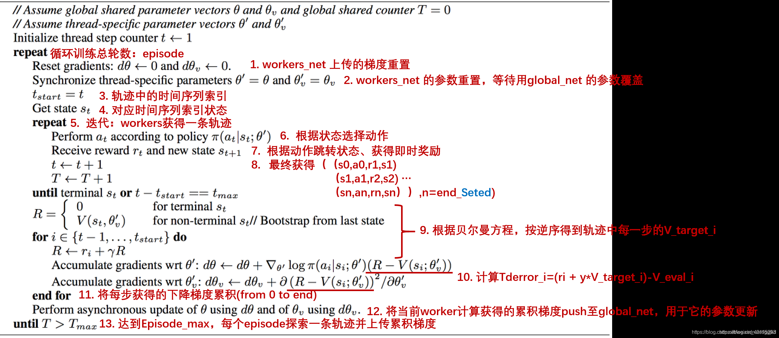
在PPO算法里,我们讲了Actor和Critic两个网络的使用,A3C的部分与它类似,它的全名是:Asynchronous advantage actor-critic译作异步优势actor-critic,它用优势函数A来估计策略梯度,由Critic估计状态价值,即:

我们展示一下A3C的伪代码,大佬写的很好,可以去看看->【强化学习】A3C原理

5

得到的梯度再进行反向传播即可。

总结

从Q学习一路讲到了AC、PPO和A3C,代码都是可以直接跑的,感兴趣的可以自己复制下来改着玩。

关于ChatGPT使用的Transformer网络,可以看这篇博文:Seq2Seq与Transformer,在早期的ChatGpt使用的是PPO算法,本文也有介绍。


深度强化学习算法
https://blog.minloha.cn/posts/212113db5ed6ef2023022101.html
作者
Minloha
发布于
2023年2月21日
更新于
2023年2月21日
许可协议