学会神经网络[2]——循环网络系列

长短期记忆与门控

长短期记忆网络::接上期博客内容,在RNN的基础上添加LSTM和GRU,只需要把神经网络的模型修改一下即可,所以我们就可以新建一个LSTM类用于测试学习效果:

1
2
3
4
5
6
7
8
9
10
11
class LSTM(nn.Module):
def __init__(self, input_size, hidden_size, output_size):
super(LSTM, self).__init__()
# 参数与RNN一样,分别为输入尺寸,隐含层尺寸并通过全连接得到输出层
self.net = nn.LSTM(input_size, hidden_size, num_layers=1, batch_first=True)
self.fc = nn.Linear(hidden_size, output_size)

def forward(self, x):
out, _ = self.net(x)
out = self.fc(out[:, -1, :])
return out

然后实现一个LSTMtry方法用于测试LSTM的学习情况:

1
2
3
4
5
6
7
8
9
def LSTMtry(train_X, train_Y, test_X, test_Y):
# 网络结构(隐含层越多信息量越多)
net = LSTM(1, 3, 1)
# 学习率变成0.2(否则学的太慢)
optims = optim.Adam(net.parameters(), lr=0.3)
# 均方误差
loss = nn.MSELoss()
train(net, train_X, train_Y, optims, loss)
test(net, test_X, test_Y, loss)

我们把上期博客的RNNtry换成LSTMtry,然后运行看看输出:

1
2
3
4
5
6
7
8
9
epoch 0, loss 0.0347
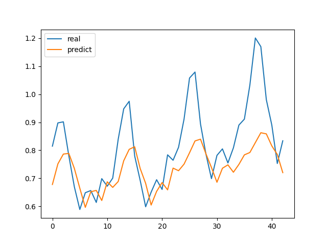
epoch 10, loss 0.0293
epoch 20, loss 0.0131
epoch 30, loss 0.0052
epoch 40, loss 0.0029
epoch 50, loss 0.0022
epoch 60, loss 0.0020
epoch 70, loss 0.0020
test loss 0.0173

运行效果如图:

1

我们看到他比RNN的损失稍微高了一点点,但是因为我们的数据只有145个,如果数据量更大的话,效果会更好。


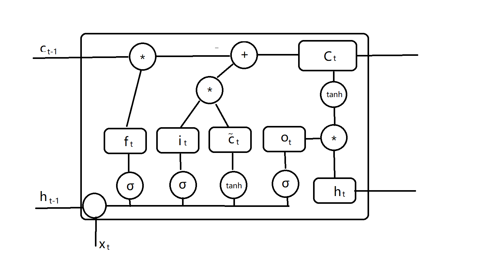
原理

为了保证能够拥有记忆时效,我们需要重新整理一下节点的结构,他需要一个输入(output),一个输出(input)和一个遗忘(forget),我们把这三部分都用门控表示,得到:
$$
i_t=\sigma(w_ix_t+U_ih_{t-1}+bi)
$$

$$
f_t=\sigma(w_fx_t+U_fh_{t-1}+b_f)
$$

i为输入门,f为遗忘门,我们计算:
$$
\hat C_t = tanh(W_cx_t+U_ch_{t-1}+b_c)
$$
然后使用上一时刻的C计算当前时刻的C:
$$
C_t=f_tC_{t-1}+i_t\hat C_t
$$
最后我们整合输出信息得到:

$$
o_t=\sigma(w_ox_t+U_oh_{t-1}+bo)
$$

$$
h_t=o_ttanh(C_t)
$$

我们很容易就看出来,这种门控结构对输出内容进行了有效的限制,这样每个神经元结构就变成了这样(画了半天,真难受)

3

c是对状态的控制,实际上LSTM仍然可以使用BPTT进行训练。在处理输入时能够同时限制学习程度,非常好的解决了长程依赖的梯度爆炸和梯度消失问题。

门控循环网络:

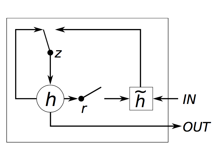
GRU(门控循环网络)的网络结果比LSTM稍微简单一点,将给一个单元都简化了一些,结构如图:

2

GRU使用了两个开关也就是重置门和更新门,使用两个单独参数控制,我们使用torch实现一个类完成GRU类:

1
2
3
4
5
6
7
8
9
10
class GRU(nn.Module):
def __init__(self, input_size, hidden_size, output_size):
super(GRU, self).__init__()
self.net = nn.GRU(input_size, hidden_size, num_layers=1, batch_first=True)
self.fc = nn.Linear(hidden_size, output_size)

def forward(self, x):
out, _ = self.net(x)
out = self.fc(out[:, -1, :])
return out

GRU在torch.nn也实现过了,参数一样,我们再完成以下GRUtry方法。

1
2
3
4
5
6
def GRUtry(train_X, train_Y, test_X, test_Y):
net = GRU(1, 3, 1)
optims = optim.Adam(net.parameters(), lr=0.1)
loss = nn.MSELoss()
train(net, train_X, train_Y, optims, loss)
test(net, test_X, test_Y, loss)

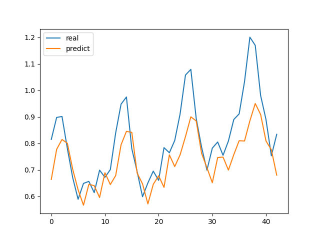
然后调用一下,当然一招鲜吃遍天。运行之后看看输出

1
2
3
4
5
6
7
8
9
epoch 0, loss 0.0336
epoch 10, loss 0.0161
epoch 20, loss 0.0033
epoch 30, loss 0.0026
epoch 40, loss 0.0027
epoch 50, loss 0.0024
epoch 60, loss 0.0021
epoch 70, loss 0.0019
test loss 0.0137

3

我们对比一下,对于少量数据用RNN即可,介于两者之间的数据量用GRU即可,数量多最好用LSTM进行学习。

到目前为止我们就已经掌握了所有神经网络的结构,那么接下来我们介绍更高级的结构和功能

序列到序列

按顺序讲,序列到序列其实算自然语言处理部分了,当然这里也不难,直接开始说,接下来我们以中英文对照数据演示,首先我们需要实现两个重要结构,对于Seq2Seq而言,我们需要将内容进行编码和解码,具体原理和流程可以看:https://blog.minloha.cn/posts/131918540f8d872023021922.html

我们需要实现Seq2Seq的编码器和解码器,我们只需要写如下内容即可,至于不将两者融合为一个Seq2Seq的原因是我们还需要对解码器进行修改。

1
2
3
4
5
6
7
8
9
10
11
12
13
14
15
16
17
18
19
20
21
22
23
24
25
26
27
28
29
30
31
32
33
34
35
36
37
38
39
40
41
42
43
44
class Encoder(nn.Module):
def __init__(self, input_size, hidden_size):
# 调用父类初始化方法
super(Encoder, self).__init__()
# 初始化必须的变量
self.hidden_size = hidden_size

self.embedding = nn.Embedding(input_size, hidden_size)
# gru的输入为三维,两个参数均指的是最后一维的大小
self.gru = nn.GRU(hidden_size, hidden_size)

def forward(self, input, hidden):
# 这里用view扩维的原因是gru必须接受三维的输入
embedded = self.embedding(input).view(1, 1, -1)
output = embedded
output, hidden = self.gru(output, hidden)
return output, hidden

def initHidden(self):
# 初始化隐层状态全为0
return torch.zeros(1, 1, self.hidden_size, device=device)


class Decoder(nn.Module):
def __init__(self, hidden_size, output_size):
super(Decoder, self).__init__()
self.hidden_size = hidden_size

self.embedding = nn.Embedding(output_size, hidden_size)
self.gru = nn.GRU(hidden_size, hidden_size)
# 经过GRU后归为一条概率向量,然后反SoftMax即可得到输出向量(利用词频反推词即可)
self.out = nn.Linear(hidden_size, output_size)
self.softmax = nn.LogSoftmax(dim=1)

def forward(self, input, hidden):
output = self.embedding(input).view(1, 1, -1)
output = F.relu(output)
output, hidden = self.gru(output, hidden)
# output的第一个1是我们用以适合gru输入扩充的, 所以用output[0]选取前面的
output = self.softmax(self.out(output[0]))
return output, hidden

def initHidden(self):
return torch.zeros(1, 1, self.hidden_size, device=device)

这里我们发现比起LSTM,我们真正的使用到了hidden层的内容,因为GRU是手动控制循环值而LSTM是利用H层自动学习的,所以我们这里使用到了GRU门控,使用GRU就必须要初始化记忆层的输出变量。接下来是对训练数据的处理,这里我抄了Github的一段代码直接可以拿到训练数据的键值对,顺便对其进行频率向量估计:

1
2
3
4
5
6
7
8
9
10
11
12
13
14
15
16
17
18
19
20
21
22
23
24
25
26
27
28
29
30
31
32
33
34
35
36
37
38
39
40
41
42
43
44
45
46
47
48
49
50
51
52
53
54
55
56
57
58
59
60
61
62
63
64
65
66
67
68
69
70
71
72
73
74
75
76
77
78
79
80
81
82
83
84
85
86
87
88
89
90
91
92
93
94
95
96
97
98
99
100
101
102
103
104
105
106
107
108
109
110
111
112
113
114
115
116
117
118
119
120
121
122
123
from io import open
import unicodedata
import re
import numpy as np

SOS_token = 0
EOS_token = 1


# 词频向量化
class ToLang:
def __init__(self, name):
self.name = name
# 结果形如 {"hello" : 3}
self.word2index = {}
# 统计每一个单词出现的次数
self.word2count = {}
self.index2word = {0: "SOS", 1: "EOS"}
# 统计训练集出现的单词数
self.n_words = 2 # SOS 和 EOS已经存在了

def addSentence(self, sentence):
# 前面是英语,后面是中文
for word in sentence.split(" "):
self.addWord(word)

def addWord(self, word):
if word not in self.word2index:
self.word2index[word] = self.n_words
self.word2count[word] = 1
# 用现有的总词数作为新的单词的索引
self.index2word[self.n_words] = word
self.n_words += 1
else:
self.word2count[word] += 1


# 将Unicode字符串转换为纯ASCII, 抄自https://stackoverflow.com/a/518232/2809427
def unicodeToAscii(s):
return ''.join(
c for c in unicodedata.normalize('NFD', s)
if unicodedata.category(c) != 'Mn'
)


# 文本修饰(去除空格, 转小写)
def normalizeString(s):
# 转码之后变小写切除两边空白
s = unicodeToAscii(s.lower().strip())
# 匹配.!?,并在前面加空格
s = re.sub(r"([.!?])", r" \1", s)
# 将非字母和.!?的全部变为空白
# s = re.sub(r"[^a-zA-Z.!?]+", r" ", s)
return s


def readLangs(lang1, lang2, reverse=False):
# 读取文件并分为几行
# 每一对句子最后会有个换行符\n
# 数据集所在位置
lines = open(r"D:\python\RL\translate\data.txt",
encoding="utf-8").read().strip().split("\n")

# 将每一行拆分成对并进行标准化
# pairs ==> [["go .","va !"],...]
pairs = [[normalizeString(s) for s in l.split("\t")] for l in lines]
pairs = np.delete(pairs, 2, axis=1)

if reverse:
pairs = [list(reversed(p)) for p in pairs]
input_lang = ToLang(lang2)
output_lang = ToLang(lang1)
else:
input_lang = ToLang(lang1)
output_lang = ToLang(lang2)

return input_lang, output_lang, pairs


# 第一个位置的语言
lang1 = "cmn"
# 第二个位置的语言
lang2 = "fra"
# 读取文件数据
input_lang, output_lang, pairs = readLangs(lang1, lang2)
# 每句话最长的长度10个字符
MAX_LENGTH = 10
# 英文前缀
eng_prefixes = (
"i am ", "i m ",
"he is", "he s ",
"she is", "she s ",
"you are", "you re ",
"we are", "we re ",
"they are", "they re "
)


# 过滤数据对,确保每句话都在规定长度内
def filterPair(p):
return len(p[0].split(' ')) < MAX_LENGTH and \
len(p[1].split(' ')) < MAX_LENGTH and \
p[1].startswith(eng_prefixes)


# 留下符合条件的
def filterPairs(pairs):
return [pair for pair in pairs if filterPair(pair)]


# 对数据进行基本处理
def prepareData(lang1, lang2, reverse=False):
input_lang, output_lang, pairs = readLangs(lang1, lang2, reverse)
print("Read %s sentence pairs" % len(pairs))
pairs = filterPairs(pairs)
print("Trimmed to %s sentence pairs" % len(pairs))
for pair in pairs:
input_lang.addSentence(pair[0])
output_lang.addSentence(pair[1])
return input_lang, output_lang, pairs


input_lang, output_lang, pairs = prepareData('eng', 'cmn', True)

在得到数据后就是我们之前说过的,利用词频进行文本向量化:

1
2
3
4
5
6
7
8
9
10
11
12
13
14
15
16
import dataTreat as dt

def indexesFromSentence(lang, sentence):
return [lang.word2index[word] for word in sentence.split(' ')]


def tensorFromSentence(lang, sentence):
indexes = indexesFromSentence(lang, sentence)
indexes.append(dt.EOS_token)
return torch.tensor(indexes, dtype=torch.long, device=device).view(-1, 1)


def tensorsFromPair(pair):
input_tensor = tensorFromSentence(dt.input_lang, pair[0])
target_tensor = tensorFromSentence(dt.output_lang, pair[1])
return input_tensor, target_tensor

接下来就是最后一步,完成数据的训练,这里我们的

1
2
3
4
5
6
7
8
9
10
11
12
13
14
15
16
17
18
19
20
21
22
23
24
25
26
27
28
29
30
31
32
33
34
35
36
37
38
39
40
41
42
43
44
45
46
47
48
49
50
51
52
53
54
55
56
57
58
59
60
61
def train(input_tensor, target_tensor, encoder, decoder, encoder_optimizer, decoder_optimizer, criterion,
max_length=dt.MAX_LENGTH):
# 初始化隐藏状态
encoder_hidden = encoder.initHidden()

# 梯度清零
encoder_optimizer.zero_grad()
decoder_optimizer.zero_grad()

input_length = input_tensor.size(0)
target_length = target_tensor.size(0)

# 初始化,等会替换
encoder_outputs = torch.zeros(max_length, encoder.hidden_size, device=device)

loss = 0

for ei in range(input_length):
encoder_output, encoder_hidden = encoder(
input_tensor[ei], encoder_hidden)
# encoder_output.size() ==> tensor([1,1,hidden_size])
encoder_outputs[ei] = encoder_output[0, 0]

# 输入为<sos>,decoder初始隐藏状态为encoder的
decoder_input = torch.tensor([[dt.SOS_token]], device=device)

decoder_hidden = encoder_hidden

# 随机决定是否采用teacher_forcing
use_teacher_forcing = True if random.random() < teacher_forcing_ratio else False

if use_teacher_forcing:
# 若采用,label作为下一个时间步输入
for di in range(target_length):
decoder_output, decoder_hidden = decoder(
decoder_input, decoder_hidden)
loss += criterion(decoder_output, target_tensor[di])
else:
# 若不用,则用预测出的作为Decoder下一个输入
for di in range(target_length):
decoder_output, decoder_hidden = decoder(
decoder_input, decoder_hidden)
topv, topi = decoder_output.topk(1)
# squeeze()进行降维
# detach将与这个变量相关的从计算图中剥离
# 从而减少内存的开销
decoder_input = topi.squeeze().detach()

loss += criterion(decoder_output, target_tensor[di])
# 若某个时间步输入为<eos>,则停止
if decoder_input.item() == dt.EOS_token:
break
# 训练时两个部分需要一起学习
loss.backward()

# 参数更新
encoder_optimizer.step()
decoder_optimizer.step()

# 返回平均loss
return loss.item() / target_length

然后我们写出trainIters进行反复多次的学习训练,这样我们就可以充分利用数据集:

1
2
3
4
5
6
7
8
9
10
11
12
13
14
15
16
17
18
19
20
21
22
23
24
25
26
27
28
29
30
31
32
33
34
35
36
37
38
39
40
41
42
43
44
45
46
47
48
49
50
51
52
53
54
55
56
57
58
59
60
61
62
63
# 获取分钟时间
def asMinutes(s):
m = math.floor(s / 60)
s -= m * 60
return '%dm %ds' % (m, s)

# 按照分钟:秒的形式返回
def timeSince(since, percent):
now = time.time()
s = now - since
es = s / percent
return '%s ' % asMinutes(s)

'''
:param encoder:编码器
:param decoder:解码器
:param n_iters:迭代次数
:param print_every:每隔多少次打印一次
:param plot_every:每隔多少次画一次图
:param learning_rate:学习率
'''


def trainIters(encoder, decoder, n_iters, print_every=100, plot_every=100, learning_rate=0.01):
start = time.time()
plot_losses = []
# 每一次重置
print_loss_total = 0
plot_loss_total = 0

# 定义优化器, Adam在当前状态下效果一般
encoder_optimizer = optim.Adam(encoder.parameters(), lr=learning_rate)
decoder_optimizer = optim.Adam(decoder.parameters(), lr=learning_rate)
# random.choice(pairs)随机选择
training_pairs = [tensorsFromPair(random.choice(dt.pairs)) for i in range(n_iters)]
criterion = nn.NLLLoss() # NLL损失函数将所有的数据点进行归一化操作,然后进入softmax计算结果

for iter in range(1, n_iters + 1):
training_pair = training_pairs[iter - 1]
input_tensor = training_pair[0]
target_tensor = training_pair[1]

loss = train(input_tensor, target_tensor, encoder,
decoder, encoder_optimizer, decoder_optimizer, criterion)

print_loss_total += loss
plot_loss_total += loss

# 若整除,就打印此时训练进度
if iter % print_every == 0:
print_loss_avg = print_loss_total / print_every
print_loss_total = 0
print('Time: %s Iterator: %d%% Acc: %.4f' % (timeSince(start, iter / n_iters), iter / n_iters * 100,
print_loss_avg))

# 若能整除,则把平均损失加入plot_loss
# 为后期画图做准备
if iter % plot_every == 0:
plot_loss_avg = plot_loss_total / plot_every
plot_losses.append(plot_loss_avg)
plot_loss_total = 0
# 学习完成后显示损失值随时间的图像
showPlot(plot_losses)

然后我们在写一个前向传播的算法,用于将我们的中文翻译为英文:

1
2
3
4
5
6
7
8
9
10
11
12
13
14
15
16
17
18
19
20
21
22
23
24
25
26
27
28
29
30
31
32
33
34
35
36
37
def evaluate(encoder, decoder, sentence, max_length=dt.MAX_LENGTH):
# 评估时停止梯度跟踪,减少内存
with torch.no_grad():
# 文本向量化(已经训练好之后才可以使用)
input_tensor = tensorFromSentence(dt.input_lang, sentence)
input_length = input_tensor.size()[0]
# 记忆层初始化
encoder_hidden = encoder.initHidden()
# 输出不能没有,并且还得放在GPU内
encoder_outputs = torch.zeros(max_length, encoder.hidden_size, device=device)

for ei in range(input_length):
encoder_output, encoder_hidden = encoder(input_tensor[ei], encoder_hidden)
encoder_outputs[ei] += encoder_output[0, 0]

# 添加文本开始标志SOS
decoder_input = torch.tensor([[dt.SOS_token]], device=device) # SOS

decoder_hidden = encoder_hidden

decoded_words = []
decoder_attentions = torch.zeros(max_length, max_length)

# 将数据按位放入Decoder内,得到我们的输出文本串(可以查看往期博客)
for di in range(max_length):
decoder_output, decoder_hidden = decoder(
decoder_input, decoder_hidden)
topv, topi = decoder_output.data.topk(1)
if topi.item() == dt.EOS_token:
decoded_words.append('<EOS>')
break
else:
decoded_words.append(dt.output_lang.index2word[topi.item()])

decoder_input = topi.squeeze().detach()

return decoded_words, decoder_attentions[:di + 1]

最后我们实现一下显示函数和main函数:

1
2
3
4
5
6
7
8
9
10
11
12
13
14
15
16
17
18
19
def showPlot(points):
plt.figure()
fig, ax = plt.subplots()
# this locator puts ticks at regular intervals
loc = ticker.MultipleLocator(base=0.2)
ax.yaxis.set_major_locator(loc)
plt.plot(points)

decoder_hidden = [10, 5, 10]

if __name__ == "__main__":
hidden_size = 256
encoder = Encoder(dt.input_lang.n_words, hidden_size).to(device)
decoder = Decoder(hidden_size, dt.output_lang.n_words).to(device)

trainIters(encoder, decoder, 20000, print_every=500)
back, att = evaluate(encoder, decoder, "我是天才")

print(back)

这样经过我们就需要40次循环我们就训练完Seq2Seq了,次数越多我们的精度越高,但是时间也越多,基本在3分钟左右。我们看一下输出内容:

1
2
3
4
5
6
7
8
9
10
11
12
13
14
15
16
17
18
19
20
21
22
23
24
25
26
27
28
29
30
31
32
33
34
35
36
37
38
39
40
41
42
43
Read 29668 sentence pairs
Trimmed to 672 sentence pairs
Time: 0m 4s Iterator: 2% Acc: 4.8165
Time: 0m 8s Iterator: 5% Acc: 4.1715
Time: 0m 12s Iterator: 7% Acc: 4.0555
Time: 0m 16s Iterator: 10% Acc: 4.1072
Time: 0m 20s Iterator: 12% Acc: 4.1130
Time: 0m 24s Iterator: 15% Acc: 4.3046
Time: 0m 28s Iterator: 17% Acc: 4.0388
Time: 0m 32s Iterator: 20% Acc: 4.1469
Time: 0m 36s Iterator: 22% Acc: 4.2702
Time: 0m 40s Iterator: 25% Acc: 4.1994
Time: 0m 44s Iterator: 27% Acc: 4.1615
Time: 0m 48s Iterator: 30% Acc: 3.9064
Time: 0m 52s Iterator: 32% Acc: 4.2069
Time: 0m 56s Iterator: 35% Acc: 4.0334
Time: 1m 0s Iterator: 37% Acc: 4.2500
Time: 1m 4s Iterator: 40% Acc: 4.2576
Time: 1m 7s Iterator: 42% Acc: 4.0754
Time: 1m 11s Iterator: 45% Acc: 3.9563
Time: 1m 15s Iterator: 47% Acc: 3.6001
Time: 1m 19s Iterator: 50% Acc: 3.7663
Time: 1m 23s Iterator: 52% Acc: 3.9296
Time: 1m 27s Iterator: 55% Acc: 3.5670
Time: 1m 30s Iterator: 57% Acc: 3.9190
Time: 1m 34s Iterator: 60% Acc: 3.8559
Time: 1m 38s Iterator: 62% Acc: 4.0905
Time: 1m 42s Iterator: 65% Acc: 4.1999
Time: 1m 46s Iterator: 67% Acc: 4.1665
Time: 1m 49s Iterator: 70% Acc: 3.9940
Time: 1m 53s Iterator: 72% Acc: 3.7515
Time: 1m 57s Iterator: 75% Acc: 3.7801
Time: 2m 1s Iterator: 77% Acc: 4.1297
Time: 2m 5s Iterator: 80% Acc: 4.2860
Time: 2m 9s Iterator: 82% Acc: 4.0266
Time: 2m 13s Iterator: 85% Acc: 4.0970
Time: 2m 16s Iterator: 87% Acc: 4.3627
Time: 2m 20s Iterator: 90% Acc: 4.5892
Time: 2m 24s Iterator: 92% Acc: 4.5988
Time: 2m 28s Iterator: 95% Acc: 4.4202
Time: 2m 32s Iterator: 97% Acc: 4.2970
Time: 2m 36s Iterator: 100% Acc: 4.2186
['she', 'is', 'a', 'inches', '.', '.', '.', '.', '.', '.']

我们发现虽然输出内容有点感觉但是精度还是不够,除了增加训练次数,又该如何优化呢?答案是增加注意力机制,具体内容可以去看https://blog.minloha.cn/posts/131918540f8d872023021922.html

1
2
3
4
5
6
7
8
9
10
11
12
13
14
15
16
17
18
19
20
21
22
23
24
25
26
27
28
29
30
31
32
33
34
35
36
37
38
39
class AttnDecoder(nn.Module):
def __init__(self, hidden_size, output_size, dropout_p=0.1, max_length=MAX_LENGTH):
super(AttnDecoder, self).__init__()
self.hidden_size = hidden_size
self.output_size = output_size
self.dropout_p = dropout_p
self.max_length = max_length

self.embedding = nn.Embedding(self.output_size, self.hidden_size)
# 因为会将prev_hidden和embedded在最后一个维度,即hidden_size,进行拼接,所以要*2
# max_length用以统一不同长度的句子分配的注意力, 最大长度句子使用所有注意力权重,较短只用前几个
self.attn = nn.Linear(self.hidden_size * 2,
self.max_length) # 输入一个大小为hidden-size*2长度的[batch-size,hidden-size*2]向量 输出为[batch-size,max_length]
self.attn = nn.Linear(self.hidden_size * 2, self.max_length)
self.attn_combine = nn.Linear(self.hidden_size * 2, self.hidden_size)
self.dropout = nn.Dropout(self.dropout_p)
self.gru = nn.GRU(self.hidden_size, self.hidden_size)
self.out = nn.Linear(self.hidden_size, self.output_size)

def forward(self, input, hidden, encoder_outputs):
embedded = self.embedding(input).view(1, 1, -1)
embedded = self.dropout(embedded)

attn_weights = F.softmax(
self.attn(torch.cat((embedded[0], hidden[0]), 1)), dim=1)
attn_applied = torch.bmm(attn_weights.unsqueeze(0),
encoder_outputs.unsqueeze(0)) # 计算两个矩阵的乘积

output = torch.cat((embedded[0], attn_applied[0]), 1) # 按列拼接 embedded[0]和embedded[1]
output = self.attn_combine(output).unsqueeze(0)

output = F.relu(output)
output, hidden = self.gru(output, hidden)

output = F.log_softmax(self.out(output[0]), dim=1)
return output, hidden, attn_weights

def initHidden(self):
return torch.zeros(1, 1, self.hidden_size, device=device)

我们这个时候就需要修改一下训练方法了:

1
2
3
4
5
6
7
8
9
10
11
12
13
14
15
16
17
18
19
20
21
22
23
24
25
26
27
28
29
30
31
32
33
34
35
36
37
38
39
40
41
42
43
44
45
46
47
48
49
50
51
52
53
54
55
56
57
58
59
60
61
62
63
64
65
66
67
68
69
70
71
72
73
74
75
76
77
78
79
80
81
82
83
84
85
86
87
88
89
90
91
92
93
94
95
96
97
98
99
100
101
102
103
104
105
106
107
108
def train(input_tensor, target_tensor, encoder, decoder, encoder_optimizer, decoder_optimizer, criterion,
max_length=dt.MAX_LENGTH):
# 初始化隐藏状态
encoder_hidden = encoder.initHidden()

# 梯度清零
encoder_optimizer.zero_grad()
decoder_optimizer.zero_grad()

input_length = input_tensor.size(0)
target_length = target_tensor.size(0)

# 初始化,等会替换
encoder_outputs = torch.zeros(max_length, encoder.hidden_size, device=device)

loss = 0

for ei in range(input_length):
encoder_output, encoder_hidden = encoder(
input_tensor[ei], encoder_hidden)
# encoder_output.size() ==> tensor([1,1,hidden_size])
encoder_outputs[ei] = encoder_output[0, 0]

# 输入为<sos>,decoder初始隐藏状态为encoder的
decoder_input = torch.tensor([[dt.SOS_token]], device=device)

decoder_hidden = encoder_hidden

# 随机决定是否采用teacher_forcing
use_teacher_forcing = True if random.random() < teacher_forcing_ratio else False

if use_teacher_forcing:
# 若采用,label作为下一个时间步输入
for di in range(target_length):

decoder_output, decoder_hidden, decoder_attention = decoder(
decoder_input, decoder_hidden, encoder_outputs)

loss += criterion(decoder_output, target_tensor[di])
else:
# 若不用,则用预测出的作为Decoder下一个输入
for di in range(target_length):
decoder_output, decoder_hidden, decoder_attention = decoder(
decoder_input, decoder_hidden, encoder_outputs)

# topk代表在所给维度上输出最大值
topv, topi = decoder_output.topk(1)
# squeeze()进行降维
# detach将与这个变量相关的从计算图中剥离
# 从而减少内存的开销
decoder_input = topi.squeeze().detach()

loss += criterion(decoder_output, target_tensor[di])
# 若某个时间步输入为<eos>,则停止
if decoder_input.item() == dt.EOS_token:
break

loss.backward()

# 参数更新
encoder_optimizer.step()
decoder_optimizer.step()

# 返回平均loss
return loss.item() / target_length


def trainIters(encoder, decoder, n_iters, print_every=100, plot_every=100, learning_rate=0.01):
start = time.time()
plot_losses = []
# 每一次重置
print_loss_total = 0
plot_loss_total = 0

# 定义优化器,经过多次运行发现SGD效果最好
encoder_optimizer = optim.SGD(encoder.parameters(), lr=learning_rate)
decoder_optimizer = optim.SGD(decoder.parameters(), lr=learning_rate)
# random.choice(pairs)随机选择
training_pairs = [tensorsFromPair(random.choice(dt.pairs)) for i in range(n_iters)]
criterion = nn.NLLLoss()

for iter in range(1, n_iters + 1):
training_pair = training_pairs[iter - 1]
input_tensor = training_pair[0]
target_tensor = training_pair[1]

loss = train(input_tensor, target_tensor, encoder,
decoder, encoder_optimizer, decoder_optimizer, criterion)

print_loss_total += loss
plot_loss_total += loss

# 若能整除,就打印此时训练进度
if iter % print_every == 0:
print_loss_avg = print_loss_total / print_every
print_loss_total = 0
print('Time: %s Iterator: %d%% Acc: %.4f' % (timeSince(start, iter / n_iters), iter / n_iters * 100,
print_loss_avg))

# 若能整除,则把平均损失加入plot_loss
# 为后期画图做准备
if iter % plot_every == 0:
plot_loss_avg = plot_loss_total / plot_every
plot_losses.append(plot_loss_avg)
plot_loss_total = 0

showPlot(plot_losses)

然后我们修改一下评估函数,让它能够显示注意力热图:

1
2
3
4
5
6
7
8
9
10
11
12
13
14
15
16
17
18
19
20
21
22
23
24
25
26
27
28
29
30
31
32
33
34
35
36
37
38
39
40
41
42
43
44
45
46
47
48
49
50
51
52
53
54
55
56
57
58
59
60
61
62
63
64
65
66
67
68
69
70
71
72
def evaluate(encoder, decoder, sentence, max_length=dt.MAX_LENGTH):
# 评估时停止梯度跟踪,减少内存
with torch.no_grad():
input_tensor = tensorFromSentence(dt.input_lang, sentence)
input_length = input_tensor.size()[0]
encoder_hidden = encoder.initHidden()

encoder_outputs = torch.zeros(max_length, encoder.hidden_size, device=device)

for ei in range(input_length):
encoder_output, encoder_hidden = encoder(input_tensor[ei], encoder_hidden)
encoder_outputs[ei] += encoder_output[0, 0]

decoder_input = torch.tensor([[dt.SOS_token]], device=device) # SOS

decoder_hidden = encoder_hidden

decoded_words = []
decoder_attentions = torch.zeros(max_length, max_length)

for di in range(max_length):
decoder_output, decoder_hidden, decoder_attention = decoder(
decoder_input, decoder_hidden, encoder_outputs)

decoder_attentions[di] = decoder_attention.data
topv, topi = decoder_output.data.topk(1)
if topi.item() == dt.EOS_token:
decoded_words.append('<EOS>')
break
else:
decoded_words.append(dt.output_lang.index2word[topi.item()])

decoder_input = topi.squeeze().detach()

return decoded_words, decoder_attentions[:di + 1]


def evaluateRandomly(encoder, decoder, n=10):
for i in range(n):
pair = random.choice(dt.pairs)
print('>', pair[0])
print('=', pair[1])
output_words, attentions = evaluate(encoder, decoder, pair[0])
output_sentence = ' '.join(output_words)
print('<', output_sentence)
print('')


# 注意力可视化
def showAttention(input_sentence, output_words, attentions):
# 用colorbar设置图
fig = plt.figure()
ax = fig.add_subplot(111)
# attentions出来之后是tensor形式,需要转换为numpy
cax = ax.matshow(attentions.numpy(), cmap='bone')
fig.colorbar(cax)

ax.set_ticks(range(len(input_sentence.split(' '))), input_sentence.split(' '))

# 在每个刻度处显示标签,刻度为1的倍数
ax.xaxis.set_major_locator(ticker.MultipleLocator(1))
ax.yaxis.set_major_locator(ticker.MultipleLocator(1))

plt.show()


def evaluateAndShowAttention(input_sentence):
output_words, attentions = evaluate(
encoder, decoder, input_sentence)
print('input =', input_sentence)
print('output =', ' '.join(output_words))
showAttention(input_sentence, output_words, attentions)

最后我们修改一下main函数即可:

1
2
3
4
5
6
7
if __name__ == "__main__":
hidden_size = 256
encoder = Encoder(dt.input_lang.n_words, hidden_size).to(device)
decoder = AttnDecoder(hidden_size, dt.output_lang.n_words).to(device)

trainIters(encoder, decoder, 20000, print_every=500)
evaluateAndShowAttention("我最帅!")

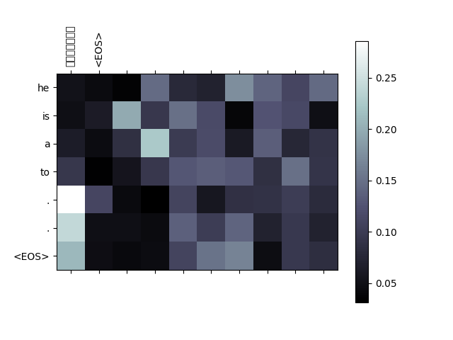
大约等待2分钟我们就可以看到输出内容了:

1
2
3
4
5
6
7
8
9
10
11
12
13
14
15
16
17
18
19
20
21
22
23
24
25
26
27
28
29
30
31
32
33
34
35
36
37
38
39
40
41
42
43
Read 29668 sentence pairs
Trimmed to 672 sentence pairs
Time: 0m 6s Iterator: 2% Acc: 3.7084
Time: 0m 11s Iterator: 5% Acc: 3.5018
Time: 0m 16s Iterator: 7% Acc: 3.3890
Time: 0m 21s Iterator: 10% Acc: 3.3418
Time: 0m 26s Iterator: 12% Acc: 3.2065
Time: 0m 31s Iterator: 15% Acc: 3.1283
Time: 0m 36s Iterator: 17% Acc: 3.0031
Time: 0m 42s Iterator: 20% Acc: 2.8943
Time: 0m 47s Iterator: 22% Acc: 2.8353
Time: 0m 53s Iterator: 25% Acc: 2.7512
Time: 0m 58s Iterator: 27% Acc: 2.6268
Time: 1m 3s Iterator: 30% Acc: 2.4636
Time: 1m 8s Iterator: 32% Acc: 2.3403
Time: 1m 13s Iterator: 35% Acc: 2.2529
Time: 1m 18s Iterator: 37% Acc: 2.0536
Time: 1m 23s Iterator: 40% Acc: 1.9667
Time: 1m 28s Iterator: 42% Acc: 1.7806
Time: 1m 33s Iterator: 45% Acc: 1.6436
Time: 1m 39s Iterator: 47% Acc: 1.5148
Time: 1m 44s Iterator: 50% Acc: 1.3833
Time: 1m 50s Iterator: 52% Acc: 1.3173
Time: 1m 56s Iterator: 55% Acc: 1.1492
Time: 2m 2s Iterator: 57% Acc: 1.0208
Time: 2m 7s Iterator: 60% Acc: 0.8369
Time: 2m 12s Iterator: 62% Acc: 0.7971
Time: 2m 17s Iterator: 65% Acc: 0.6642
Time: 2m 22s Iterator: 67% Acc: 0.6291
Time: 2m 28s Iterator: 70% Acc: 0.5314
Time: 2m 33s Iterator: 72% Acc: 0.4829
Time: 2m 38s Iterator: 75% Acc: 0.4303
Time: 2m 43s Iterator: 77% Acc: 0.3285
Time: 2m 48s Iterator: 80% Acc: 0.2829
Time: 2m 53s Iterator: 82% Acc: 0.2468
Time: 2m 59s Iterator: 85% Acc: 0.2233
Time: 3m 4s Iterator: 87% Acc: 0.1972
Time: 3m 9s Iterator: 90% Acc: 0.1789
Time: 3m 14s Iterator: 92% Acc: 0.1774
Time: 3m 20s Iterator: 95% Acc: 0.1612
Time: 3m 25s Iterator: 97% Acc: 0.1309
Time: 3m 30s Iterator: 100% Acc: 0.1419
['i', 'am', 'cool', '', '.', '.', '.', '.', '.', '.']

热图:

4

总结

本期博客介绍了循环神经网络系列内容,当然Seq2Seq内容过长,学起来难度不小,所以需要反复复习才可以精通,基础内容也不能拉下,共勉!


学会神经网络[2]——循环网络系列
https://blog.minloha.cn/posts/122633e3065d622024022616.html
作者
Minloha
发布于
2024年2月26日
更新于
2024年3月1日
许可协议